If a Funciton is Continuous Does It Have a Continuous Inverse Laplace
The following Laplace transform table helps to solve the differential equations for different functions:
Laplace Transform of Differential Equation
The Laplace transform is a well established mathematical technique for solving a differential equation. Many mathematical problems are solved using transformations. The idea is to transform the problem into another problem that is easier to solve. On the other side, the inverse transform is helpful to calculate the solution to the given problem.
For better understanding, let us solve a first-order differential equation with the help of Laplace transformation,
Consider y'- 2y = e3x and y(0) = -5. Find the value of L(y).
First step of the equation can be solved with the help of the linearity equation:
L(y' – 2y] = L(e3x)
L(y') – L(2y) = 1/(s-3)
(because L(eax) = 1/(s-a))
L(y') – 2s(y) = 1/(s-3)
sL(y) – y(0) – 2L(y) = 1/(s-3)
(Using Linearity property of the Laplace transform)
L(y)(s-2) + 5 = 1/(s-3) (Use value of y(0) ie -5 (given))
L(y)(s-2) = 1/(s-3) – 5
L(y) = (-5s+16)/(s-2)(s-3) …..(1)
here (-5s+16)/(s-2)(s-3) can be written as -6/s-2 + 1/(s-3) using partial fraction method
(1) implies L(y) = -6/(s-2) + 1/(s-3)
L(y) = -6e2x + e3x
Step Functions
The step function is often called the Heaviside function, and it is defined as follows:
\(\begin{array}{l}u_{c}(t)= \left\{\begin{matrix} 0 & if\ t<c \\ 1 & if\ t\geq c \end{matrix}\right.\end{array} \)
The step function can take the values of 0 or 1. It is like an on and off switch. The notations that represent the Heaviside functions are u c (t) or u(t-c) or H(t-c)
Bilateral Laplace Transform
The Laplace transform can also be defined as bilateral Laplace transform. This is also known as two-sided Laplace transform, which can be performed by extending the limits of integration to be the entire real axis. Hence, the common unilateral Laplace transform becomes a special case of Bilateral Laplace transform, where the function definition is transformed is multiplied by the Heaviside step function.
The bilateral Laplace transform is defined as:
\(\begin{array}{l}F(s)=\int_{-\infty }^{+\infty }e^{-st}f(t)dt\end{array} \)
The other way to represent the bilateral Laplace transform is B{F}, instead of F.
Inverse Laplace Transform
In the inverse Laplace transform, we are provided with the transform F(s) and asked to find what function we have initially. The inverse transform of the function F(s) is given by:
f(t) = L -1 {F(s)}
For example, for the two Laplace transform, say F(s) and G(s), the inverse Laplace transform is defined by:
L -1 {aF(s)+bG(s)}= a L -1 {F(s)}+bL -1 {G(s)}
Where a and b are constants.
In this case, we can take the inverse transform for the individual transforms, and add their constant values in their respective places, and perform the operation to get the result.
Also, check:
- Laplace Transform Calculator
- Inverse Laplace Transform
Convolution Integrals
If the functions f(t) and g(t) are the piecewise continuous functions on the interval [0, ∞), then the convolution integral of f(t) and g(t) is given as:
(f * g) (t) = 0 ∫ t f(t-T) g(T)dT
As, the convolution integral obey the property, (f*g)(t) = (g*) (t)
We can write, 0∫t f(t-T) g(T)dT = 0∫t f(T) g(t-T)dt
Thus, the above fact will help us to take the inverse transform of the product of transforms.
(i.e.) L(f*g) = F(s) G(s)
L -1 {F(s)G(s)} = (f*g)(t).
Laplace Transform in Probability Theory
In pure and applied probability theory, the Laplace transform is defined as the expected value. If X is the random variable with probability density function, say f, then the Laplace transform of f is given as the expectation of:
L{f}(S) = E[e -sX ], which is referred to as the Laplace transform of random variable X itself.
Applications of Laplace Transform
- It is used to convert complex differential equations to a simpler form having polynomials.
- It is used to convert derivatives into multiple domain variables and then convert the polynomials back to the differential equation using Inverse Laplace transform.
- It is used in the telecommunication field to send signals to both the sides of the medium. For example, when the signals are sent through the phone then they are first converted into a time-varying wave and then superimposed on the medium.
- It is also used for many engineering tasks such as Electrical Circuit Analysis, Digital Signal Processing, System Modelling, etc.
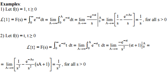
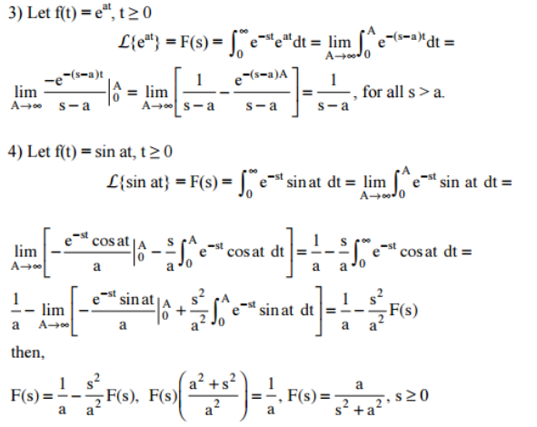
Laplace Transform Examples
Below examples are based on some important elementary functions of Laplace transform.
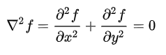
Laplace Equation
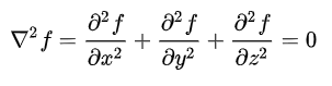
Laplace's equation, a second-order partial differential equation, is widely helpful in physics and maths. The Laplace equation states that the sum of the second-order partial derivatives of f, the unknown function, equals zero for the Cartesian coordinates. The two-dimensional Laplace equation for the function f can be written as:
The Laplace equation for three-dimensional coordinates can be represented as:
Download BYJU'S-The Learning App and get personalised videos to understand the mathematical concepts.
Frequently Asked Questions on Laplace Transform- FAQs
What is the use of Laplace Transform?
The Laplace transform is used to solve differential equations. It is accepted widely in many fields. We know that the Laplace transform simplifies a given LDE (linear differential equation) to an algebraic equation, which can later be solved using the standard algebraic identities.
How do you calculate Laplace transform?
The steps to be followed while calculating the Laplace transform are:
Step 1: Multiply the given function, i.e. f(t) by e^{-st}, where s is a complex number such that s = x + iy
Step 2; Integrate this product with respect to the time (t) by taking limits as 0 and ∞.
This process results in Laplace transformation of f(t), and is denoted by F(s).
What is the Laplace method?
The Laplace transform (or Laplace method) is named in honor of the great French mathematician Pierre Simon De Laplace (1749-1827). This method is used to find the approximate value of the integration of the given function. Laplace transform changes one signal into another according to some fixed set of rules or equations.
What are the properties of Laplace Transform?
The important properties of Laplace transform include:
Linearity Property: A f_1(t) + B f_2(t) ⟷ A F_1(s) + B F_2(s)
Frequency Shifting Property: es0t f(t)) ⟷ F(s – s0)
nth Derivative Property: (d^n f(t)/ dt^n) ⟷ s^n F(s) − n∑i = 1 s^{n − i} f^{i − 1} (0^−)
Integration: t∫_0 f(λ) dλ ⟷ 1⁄s F(s)
Multiplication by Time: T f(t) ⟷ (−d F(s)⁄ds)
Complex Shift Property: f(t) e^{−at} ⟷ F(s + a)
Time Reversal Property: f (-t) ⟷ F(-s)
Time Scaling Property: f (t⁄a) ⟷ a F(as)
What is the Laplace transform of sin t?
The Laplace transform of f(t) = sin t is L{sin t} = 1/(s^2 + 1). As we know that the Laplace transform of sin at = a/(s^2 + a^2).
mccueabouldepard1969.blogspot.com
Source: https://byjus.com/maths/laplace-transform/
0 Response to "If a Funciton is Continuous Does It Have a Continuous Inverse Laplace"
Post a Comment